
Table of Contents
Study participants
ProDiGY is a collaborative effort to understand the genetic predisposition of youth-onset T2D using multi-ethnic diabetes cases from SEARCH, TODAY and the TODAY Genetics study as previously described4,9. In brief, SEARCH is a longitudinal observation study on youth-onset diabetes in the United States (diagnosed at under 20 years of age) initiated in 2000 (ref. 26). The TODAY study is a randomized clinical trial that enroled participants with T2D age 10–17 years between 2004 and 2009 (ref. 27). Participants were diagnosed with T2D before 18 years of age; had BMI ≥ 85th percentile for age, sex and height; and did not have evidence of type 1 diabetes (negative of pancreatic islet autoantibodies and positive for C-peptide level greater than 0.6 ng ml−1). The TODAY Genetics study is ancillary to the TODAY clinical trial and enroled additional cases with similar criteria to the TODAY study.
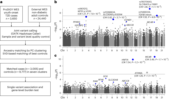
In the current study, we investigated a total of 3,650 individuals with youth-onset T2D (553 participants from SEARCH, 526 from TODAY and 2,571 from the TODAY Genetics study). Participants with confirmed MODY and those suspected to have MODY on the basis of clinical judgement (that is, autoantibody negative and not overweight or obese) at study enrolment were excluded. Non-diabetic adult control samples were derived from the previously published6 AMP-T2D-GENES whole-exome sequence analysis, which involved 29,791 T2D cases and 24,440 control participants from five major ancestries. Criteria for inclusion as non-diabetic control participants were study-specific and were described previously6. After matching cases and control participants on the basis of their genetic background as described below, there were 3,005 participants in total with youth-onset T2D and 9,777 control participants available for genetic association testing. The effective sample size of this study, defined as 4 × ncases × ncontrols/(ncases + ncontrols), was 9,194. In the case group, BMI was available in 881 participants whereas fasting C-peptide and age at diagnosis was available for 2,960 and 3,005 participants, respectively.
Whole-exome sequence data generation
ProDiGY whole-exome sequencing data were generated as part of a previously published study and therefore used identical variant calling, quality control procedures and variant annotation procedures as described previously6. In brief, genomic DNA was extracted form peripheral leucocytes and was sheared, ligated with Illumina barcoded sequence adaptors and amplified. Whole-exome in-solution hybrid capture was done with the Illumina Rapid Capture Exome enrichment kit (target region size 38 Mb). The enriched libraries were quantified, normalized and subjected to massive parallel sequencing using the HiSeq 4000 Sequencing system. Sequencing reads were aligned to the human genome build hg19 using the Picard (https://broadinstitute.github.io/picard/), Burrows–Wheeler Alignment28 and Genome Analysis Toolkit29 software. We excluded duplicate or sex-discordant samples on the basis of identity-by-descent analysis, as well as lower call rate samples in any pair with an identity-by-descent value greater than 0.3.
Matching external control participants
For matching ProDiGY samples to external control participants, we first used genetic principal components of 5,496 linkage disequilibrium pruned autosomal variants to cluster all case and control samples into ancestry groups. Clustering was performed using MClust Gaussian model fitting as implemented in the SVDFunctions package (https://github.com/alexloboda/SVDFunctions). We then applied a singular-value decomposition (SVD)-based method11 to find the best set of control participant-matching cases within each ancestry group. Specifically, left singular vectors of the case genotype matrix were used to compute the estimated residual norm for every prospective control and generate a ranking of the degree to which they represented cases within their ancestry group11. For every control residual vector norm threshold, an association test (between cases and controls above the threshold) was performed and a genomic inflation factor was estimated11. The largest control set that provided a genomic inflation factor less than 2.0 and control sample size of more than 500 were chosen for each ancestry cluster using the selectControls() function in the SVDFunctions package. There was a total of seven clusters (Extended Data Fig. 1) that had genomic inflation factors between 1.03 and 1.75, and the final genomic inflation factor after meta-analysis was 1.15.
Variant annotation
We annotated variants using the ENSEMBL VEP (v.87)30. Annotations were generated for all ENSEMBL transcripts, using the –flag-pick allele option to designate a ‘best guess’ annotation to each variant on the basis of a set of ordered criteria for transcripts31: transcript support level (that is, supported by mRNA), biotype (that is, protein_coding), APPRIS isoform annotation (that is, principal), the deleteriousness of annotation (that is, preference given to transcripts with higher impact annotations), consensus coding sequence database status of the transcript32 (that is, a high-quality transcript set) and canonical status of the transcript and transcript length (that is, longer is preferred). We used the VEP LofTee (https://github.com/konradjk/loftee) and dbNSFP (v.3.2)33 plugins to yield additional bioinformatic predictions of variant deleteriousness. From the dbNSFP plugin, we extracted annotations from 15 distinct bioinformatic algorithms along with the mCAP algorithm34. Since these annotations were not transcript specific, we allocated them to all transcripts for the sake of downstream analysis. All single-variant analyses described in the paper use the ‘best guess’ annotation for each variant.
Statistical analysis and reproducibility
To investigate genetic risk factors for youth-onset T2D, we conducted a series of analyses. These included single-variant and gene-level rare variant association studies, as detailed below. Additionally, we carried out gene-set enrichment analysis, examined LVE by these variants and analysed the individual-level genetic risk on the basis of common and rare variants also as described below.
Single-variant association analysis
We performed single-variant association tests using Firth’s penalized logistic regression as implemented in Hail v.0.2.43 (https://github.com/hail-is/hail/releases/tag/0.2.43). Association testing was done for cases and matched control participants in each of the seven ancestry clusters, adjusting for genetic principal components (PC1–PC10) significantly associated with youth-onset T2D after Bonferroni correction (P < 0.005). For each cluster, we performed additional variant quality control by including only biallelic autosomal variants with (1) P ≥ 0.0001 for variant differential missingness between cases and control participants, (2) P ≥ 0.0001 for Hardy–Weinberg equilibrium, (3) (alternate allele genotype quality score (GQ) ≥ 95, call rate (CR) ≥ 0.95) or (alternate allele GQ < 95, CR ≥ 0.99, P ≥ 0.001 for variant differential missingness between cases and control participants, P ≥ 0.001 for Hardy–Weinberg equilibrium), (4) variant read depth greater than or equal to 50, or (variant read depth less than 50, P ≥ 0.001 for variant differential missingness between cases and control participants, P ≥ 0.001 for Hardy–Weinberg equilibrium, P ≥ 0.001 for Hardy–Weinberg equilibrium in cases, P ≥ 0.001 for Hardy–Weinberg equilibrium in controls), (5) Firth P ≥ 0.05 × P value for Fisher’s exact test and (6) a passing random forest filter of gnomAD exomes and genomes. We confirmed that these filters resulted in a well-calibrated test statistic for each cluster without significant inflation through inspection of quantile–quantile plots (Extended Data Fig. 2). Among the variants remaining within each cluster, we then conducted a seven-way inverse-variance weighted meta-analysis using METAL35 (some variants were present in fewer than seven clusters due to quality control exclusions). Exome-wide significance for coding variants13 was set as P < 4.3 × 10⁻⁷ and genome-wide significance for non-coding variants was set as P < 5.0 × 10⁻⁸. For downstream tests of concordance between youth-onset T2D effect sizes in ProDiGY and adult-onset T2D effect sizes in AMP-T2D-GENES, a binomial test was performed.
Gene-level association analysis
Gene-level association analysis was conducted as previously described with minor modifications6. For each gene, we grouped variants into seven nested ‘masks’6,36 on the basis of 16 different bioinformatic predictions of variant deleteriousness33. These seven masks were (from most stringent to least stringent): (1) LOFTEE (LOFTEE high confidence), (2) 16 out of 16 (pass 11 out of 11 criteria, VEST3 > 90%, CADD > 90%, DANN > 90%, Eigen-raw > 90% and Eigen-principal component-raw > 90%), (3) 11 out of 11 (pass 5 out of 5 but fail 16 out of 16 criteria, FATHMM pred = D, FATHMM-MKL pre = D, PROVEAN pred = D, metaSVM pred = D, MetaLR = D and MCAP > 0.025), (4) 5 out of 5 (fail 11 out of 11 criteria, PolyPhen HDIV pred = D, PolyPhen HVAR pred = D, SIFT pred = del, LFT pred = D and MutTaster pred = D/A), (5) 5 out of 5 + LOFTEE LC 1% (pass 5 out of 5 criteria or VEP Impact = HIGH, LOFTEE low confidence and Max MAF < 1%), (6) 1 out of 5 1% (fail 5 out of 5 criteria, VEP Impact = MOD and Max MAF < 1%) and (7) 0 out of 5 1% (fail 1 out of 5 criteria, VEP Impact = MOD and Max MAF < 1%). For each gene and mask, up to three groupings of alleles were generated on the basis of different transcript sets of the gene. The variants included in each unique mask for the top 20 gene-level associations’ best guess transcript are displayed in Supplementary Table 4.
Before running gene-level association tests, we applied the same variant quality control filters as for single-variant association analysis. For each mask, we then conducted burden analyses (in which an individual’s phenotype is regressed on the number of variants in the mask carried by the individual) using Firth’s penalized logistic regression, as implemented in EPACTS v.3.2.4 (https://genome.sph.umich.edu/wiki/EPACTS). Regressions were adjusted for ten principal components and seven ancestry clusters. The seven P values for each gene mask and up to three P values for transcript sets were consolidated by a minimum P value test, in which a gene was assigned its smallest P value across masks after correction for the effective number of independent masks (as estimated by the gene-specific correlation of variants across masks6,12). As this procedure produced one P value per gene, the gene-level significance threshold was set to P < 2.6 × 10⁻⁶ (P = 0.05/19,020 genes).
Accounting for sample size differences, control sample overlap and winner’s curse in effect size comparisons
Many of our analyses compared properties of associations across different datasets (ProDiGY versus AMP-T2D-GENES) and across frequency ranges (rare versus common). These properties included the proportion of associations in one study observed in the other, the consistency of effect size directions, the relative effect size magnitudes and the LVE. We applied a series of analytical and simulation-based adjustments for the potential confounders as below.
For comparisons of variant effect sizes between ProDiGY and AMP-T2D-GENES, we adjusted for control sample overlap and winner’s curse. We first simulated 1,000 replicates of two association studies (under the null model): one with the same number of cases and control participants as ProDiGY, one with the same number of cases and control participants as AMP-T2D-GENES and with the studies sharing the same number of control participants as the empirical studies. The number of variants and their frequencies were matched to the number empirically observed for ProDiGY. Genotypes were simulated as binomial random variables, cases had phenotypes set to 0 and controls had phenotypes set to one, and effect sizes and P values were generated via linear regression. We used the results of these studies to calculate expected values (and standard errors) for two quantities of interest in our analyses: effect size concordances between the studies, and fraction of variants that had larger effect sizes in one study as opposed to the other.
For analyses in which variants were ascertained on the basis of P values in either AMP-T2D-GENES or ProDiGY, we corrected for winner’s curse in these calculations by re-conducting these simulations for sets of variants chosen on the basis of either (1) their rank in the P value distribution for one of the two studies or (2) a P value threshold. This analysis accounted for differences in sample size (and hence winner’s curse) between the studies, depending on whether we drew simulated variants on the basis of their P values in the larger or smaller simulated study.
For analyses in which variants were not ascertained on the basis of their association results, and therefore not subject to winner’s curse, we simply drew a set at random from the simulations. For example, the ‘known diabetes gene set‘ was curated on the basis of various sources including genes causing monogenic diabetes, genes for T2D drug targets, genes identified in GWAS to harbour causal coding variants, genes of monogenic obesity and mouse diabetes genes as described in Supplementary Table 8.
Accounting for winner’s curse for other analyses
For all other analyses in which we analysed variants selected on the basis of their observed P values in ProDiGY or AMP-T2D-GENES, we applied a previously developed winner’s curse correction to reduce the bias in effect size estimates37. Specifically, the likelihood of the observed effect size, conditional on achieving a given association threshold, is given by:
$$P\left({\beta }_{\mathrm{obs}}|{\beta }_{\mathrm{true}}\right)=\frac{\frac{1}{s}\phi \left(\frac{{{\beta }_{\mathrm{obs}}-\beta }_{\mathrm{true}}}{s}\right)}{\Phi \left(\frac{{\beta }_{\mathrm{true}}}{s}-c\right)+\Phi \left(\frac{{-\beta }_{\mathrm{true}}}{s}-c\right)}1\left(\left|\frac{{\beta }_{\mathrm{obs}}}{s}\right|\ge c\right)$$
where \({\beta }_{\mathrm{obs}}\) is the observed effect size, \({\beta }_{\mathrm{true}}\) is the winner’s curse corrected effect size (which we used in our downstream analyses), \(c\) is the z score threshold (corresponding to the P value threshold) used to ascertain variants for the analysis, s is the standard error of \({\beta }_{\mathrm{obs}}\), \(\phi\) is the normal density distribution and \(\Phi\) is the normal cumulative distribution. We obtained \({\beta }_{\mathrm{true}}\) estimates using maximum likelihood (as implemented by numerical optimization). We obtained confidence interval estimates, under the asymptotic chi-squared approximation for the log-likelihood, by solving for the log-likelihood values that yielded the appropriate chi-squared distribution quantiles.
When calculating properties of a set of variants subject to winner’s curse (for example, total LVE explained), we obtained confidence intervals by sampling from the distributions of \({\beta }_{\mathrm{obs}}\). Specifically, for each sample, we drew a value of \(\widetilde{{\beta }_{\mathrm{obs}}}\) for each variant by sampling from a chi-square distribution and then numerically finding the value of \(\widetilde{{\beta }_{\mathrm{obs}}}\) with likelihood equal to the sampled value. We then calculated the property of interest (for example, LVE) using the sampled \(\widetilde{{\beta }_{\mathrm{obs}}}\) values. We repeated this process 1,000 times and used the results to obtain desired confidence intervals.
Gene-set enrichment analysis and gene-set classification
We conducted two types of enrichment analysis: one that evaluated the overlap of the set with the strongest gene-level associations, and the other that evaluated the entire set of gene-level P values in the set. For the first analysis, we analysed 5,071 Human Phenotype Ontology14 database gene sets as specified in MSigDB16. We used a hypergeometric test, as implemented in gene-set enrichment analysis (https://www.gsea-msigdb.org/gsea/index.jsp)38, to evaluate the overlap of each gene set with the top 50 genes from our ProDiGY analysis (that is, the 50 genes with the lowest P values according to the minimum P value test). We considered a gene set as significant if it achieved false discovery rate q value less than 0.01 on the basis of the Benjamini and Hochberg method.
Out of the 38 gene sets that showed significant over-representation of the top 50 gene-level association signals, 25 gene sets were defined by Human Phenotype Ontology terms including ‘diabetes’, ‘hyperglycaemia’, ‘glucose’, ‘HbA1c’, ‘insulin’, ‘pancreas’, ‘c peptide’, ‘overweight’ and ‘waist’. We considered these to be involved in metabolic phenotypes of T2D and further subdivided them into clusters of ‘β-cell function’, ‘obesity’ and ‘other T2D’ by independent analysis of two investigators. In cases of any conflicts, consensus was reached through discussion and agreement.
We subjected these 25 gene sets, as well as six others (‘Monogenic OMIM + neonatal diabetes’, ‘Monogenic primary’, ‘Monogenic secondary’, ‘Monogenic obesity’, ‘Lipodystrophy’ and ‘Type 1 diabetes’) described in Supplementary Table 10, to a second gene-set analysis. For each set we selected 50-fold matched control genes with similar numbers and frequencies of variants within them (following a previously described procedure6). We then performed a one-sided Wilcoxon rank-sum test to assess whether genes in the curated gene set had significantly lower P values (as calculated by the minimum P value test) than the matched control genes. When gene sets were combined into ‘obesity’, ‘β-cell function’, ‘other’ and ‘overall’, we selected fivefold matched control genes. Fold enrichment represents the fraction of genes in the gene set that are within the top 10% of associations with youth-onset T2D when compared to background genes.
LVE analysis
For all calculations of genetic LVE (for a variant or for a gene), we used a previously reported formula that incorporates three genotypes (AA, Aa, aa), their population frequencies and their relative risks (1, RR1 and RR2)39. We calculated values for this formula on the basis of observed allele frequency (MAF for single-variant association and cumulative allele frequency for gene-level association) and observed variant or gene effect size (which we converted to relative risk assuming a diabetes prevalence of 8% under an additive genetic model); the extension from variants to genes requires some approximations and assumptions (similar to those of a burden test) and has been previously applied and described in detail6.
To compare rare and common variant genetic architectures within ProDiGY, we performed several LVE calculations for both rare variant gene-level associations and common variants. Our primary analysis was to compare LVE explained by ten gene-level associations of tier 3 genes (MC4R, HNF1A, GCK, SLC30A8, ABCC8, PAM, RFX6, GHRL, HESX1, SIX3, excluding ATXN2L as its association was driven by a common variant) to the ten strongest validated common variant associations of adult-onset T2D (rs2237897, rs7903146, rs150111048, rs1421085, rs4929965, rs11709077, rs10882101, rs1708302, rs738408, rs10937721). As a secondary sensitivity analysis, we conducted additional comparisons using different sets of associations: (1) three gene-level associations and six common variant associations that reached exome-wide significance, (2) the top 25 gene-level associations in ProDiGY and the top 25 common variant associations in ProDiGY and (3) the 38 gene-level associations of tier 4 genes and the top 38 common variant associations in AMP-T2D-GENES.
We also compared the LVE estimates for youth-onset T2D obtained using ProDiGY to those for adult-onset T2D using AMP-T2D-GENES, focusing on rare and common variants. For tier 3 (n = 10) and tier 4 (n = 38) genes and common variants, the identical genes and variants used in ProDiGY were used to calculate LVE for adult-onset T2D (AMP-T2D-GENES). For exome-wide significant genes and variants, as well as the top 25 genes and variants, the corresponding genes and variants that met the criteria (exome-wide significant or top 25) in adult-onset T2D were used to compute LVE. These exome-wide or top 25 genes and variants underwent winner’s curse correction for both ProDiGY and AMP-T2D-GENES, as detailed below.
These comparisons were subject to two sources of bias and confounding. First, using observed variant or gene effect size estimates upwardly biases LVE calculations, due to uncertainty in effect size estimation. This is particularly problematic when comparing variants of different frequencies (which produce standard errors of different magnitudes) and when comparing variants or genes across studies (for example, ProDiGY and AMP-T2D-GENES) that have substantially different sample sizes. A second source of bias is winner’s curse: many of our analysed variant or gene sets were selected on the basis of achieving a significant association in either ProDiGY or AMP-T2D-GENES. This upwardly biases LVE estimates to a degree that is influenced by both the power of the study and the ascertainment criteria for the set.
We therefore first extended our LVE formula to account for uncertainty in the estimate of effect size for a variant or gene (which upwardly biases LVE estimates). As has been shown previously40, for quantitative traits the observed variance explained is approximately equal to the true variance explained plus the square of the standard error in the effect size estimate. We therefore calculated LVE by (1) calculating an upwardly biased LVE estimate using the estimated variant or gene effect size; (2) calculating an LVE correction term using the square of the estimated variant or gene standard error and (3) subtracting the correction term from the upwardly biased estimate. We verified using simulations that this calculation produced unbiased LVE estimates under the null.
For gene-level LVE estimation, we used effect size estimates from the mask achieving the lowest P value. We used standard errors corrected for the effective number of masks: we applied our minimum P value procedure to convert the original mask P value to a corrected P value, we converted this P value to a z score under the normal distribution, and we then computed the standard error that would produce this z score given the mask-level effect size.
We finally ensured that we corrected all LVE estimates for winner’s curse by applying our winner’s curse correction (above) to the effect size estimates for variants or genes. This only affected variant or gene sets ascertained on the basis of their observed P values or ranks within ProDiGY (or AMP-T2D-GENES); sets ascertained by other criteria were not subjected to winner’s curse correction.
Common and rare variant scores
To investigate individual-level genetic heterogeneity within ProDiGY, we sought to compare the phenotypes of cases ‘due predominantly to common variants’ to those of cases ‘due predominantly to rare variants’. Ideally, we would identify such individuals by constructing youth-onset T2D common variant and rare variant polygenic scores in an independent cohort, and then applying them to ProDiGY. However, no such independent cohort exists. Therefore, we approximated these by defining rare and common variant ‘contribution scores’ using association statistics within ProDiGY, correcting for winner’s curse in situations when variants were ascertained on the basis of ProDiGY P values.
If we were to use these scores to predict risk of youth-onset T2D in ProDiGY, we would be subject to circularity and overfitting due to overlapping training and test data. However, as we only evaluated phenotypes orthogonal to T2D (for example, C-peptide, age of diagnosis, BMI), we reasoned that overfitting would be less of a concern (if any). Nonetheless, we use the term ‘contribution score’ rather than ‘polygenic risk score’ to avoid any implication that we are attempting to apply these in the traditional risk prediction setting.
For the common variant contribution score, we used the same method as previously described for polygenic score4. Briefly, we constructed a common variant score for each ancestry using risk alleles and their effect sizes from previously reported T2D GWAS41 that did not include samples from ProDiGY and standardized the scores to z scores. These z scores were converted to β values on the basis of the effect size in each ancestry4. The β values for a one standard deviation increase in common variant score was 0.89, 0.37 and 0.91 for Europeans, African Americans and Latinos, respectively4. As these scores were constructed from data independent to ProDiGY, they are unbiased ‘polygenic scores’ for ProDiGY samples rather than simply ‘contribution scores’.
For the rare variant contribution score, we used 46 genes that met two criteria: (1) they were included in at least one of the 25 significantly enriched gene sets and were related to metabolic phenotypes of diabetes, and (2) had at least nominally significant gene-level association with youth-onset T2D (P < 0.05). We then applied a previous procedure42 for constructing a polygenic score from variants in each mask, applying the ‘unique’ fitting procedure; briefly, each variant is assigned a weight equal to the estimated effect size of the specific mask that contains it, with the effect size computed after removing variants in the mask that were present in more stringent masks. As the genes in this score were selected on the basis of ProDiGY P values, we applied a winner’s curse correction (above) to their effect sizes before constructing the score. Combined rare and common variant contribution scores were generated by adding the common variant score and rare variant score for each sample.
We conducted two analyses using these scores. First, we compared the relative number of samples that had common, rare and combined scores above OR ≥ 3. Second, we tested each rare and common score for association with age at diabetes diagnosis, BMI z score and log10(C-peptide) level in ProDiGY cases using linear regression.
Ethics statement
All clinical research was approved by the institutional review board of the participating cohort and written informed consent was obtained from each study participant (and their parent or guardian if the participant was under 18 years of age). All clinical investigations were conducted according to the Declaration of Helsinki.
Reporting summary
Further information on research design is available in the Nature Portfolio Reporting Summary linked to this article.